You are here: Home >> Beginner’s Guide >> Betting Strategies >> Maximising Expected Risk to Return Ratio
The following discussion is based on a previous article: Maximising Expected Return to Risk Ratio. Most of the content has been sourced from chapter 20 in the book Paul Wilmott introduces quantitative finance, by Paul Wilmott.
Maximising Expected Return
The strategy that most punters implicitly use is to maximise expected return, which works as follows. Consider the ‘high bat’ odds for Australia’s first innings in a test match. We assess the options and determine our perceived probability that each player will win. We then run the calculation (ODDS * PERCEIVED_PROBABILITY) – 1 to determine the expected return for each pick.
| Batsman | Bookmaker Odds | Perceived Probability | Expected Return |
|---|---|---|---|
| Ricky Ponting | 4.00 | 20% | -20% |
| Simon Katich | 5.00 | 23% | 15% |
| Phillip Hughes | 5.25 | 15% | -21% |
| Michael Clarke | 5.50 | 22% | 21% |
| Michael Hussey | 8.00 | 8% | -52% |
| Marcus North | 7.50 | 6% | -55% |
| Brad Haddin | 10.00 | 5% | -50% |
| Mitchell Johnson | 31.00 | 1% | -69% |
| Nathan Hauritz | 81.00 | 0% | -100% |
| Peter Siddle | 201.00 | 0% | -100% |
| Ben Hilfenhaus | 251.00 | 0% | -100% |
| Total probability | 100% | ||
Based on these probabilities we would back Michael Clarke because he provides the highest expected return. The expected return for backing Clarke is 21% with a standard deviation of 228% (the methodology for calculating standard deviation will be discussed shortly). Note that if none of the expected returns are positive, our best strategy is to not place a wager.
The problem with maximising expected return, however, is that it pays no attention to risk. Measuring risk in a sports betting context may seem a foreign concept, so let’s first consider risk in the context of investing. Consider a high interest savings account that pays a guaranteed 6% interest per annum. If you expect the share market to also grow at 6% per annum you would always choose the interest account. This is because your earnings are virtually guaranteed with the savings account, but highly uncertain in the share market. Even if you expect a 7% return in the share market you would still likely prefer the interest account because the extra expected return is not worth the risk. Using the maximising expected return strategy, you would always choose the share market even if it returns only 0.1% more than an interest account because the strategy does not account for risk. What we need is a strategy that takes risk into account when making a decision.
Maximising Expected Return to Risk Ratio
The following strategy moderates your exposure to risk and it is a mathematically superior strategy to simply maximising your expected return. It maximises your expected return to risk ratio. Note the use of the word ‘expected’ because this involves determining your own probabilities for each of the expected outcomes. You don’t know these probabilities with certainty – they are simply based on your expectations.
Consider again at the ‘high bat’ market for Australia’s first innings in a test match.
If we place an equal wager on each player, the expected return equals the average of the individual returns (-20% + 15% + …) / 11. Based on our probabilities from the table above, this equals -48%. If we wish to maximize expected return we would bet on Clarke to provide an expected return of 21%. The problem with this strategy is it involves a considerable amount of risk. Risk can be simply thought of as uncertainty, and in this case, it is measured by the standard deviation of returns. The standard deviation for backing Clarke is 228%, which is huge. The reward to risk ratio for this wager is 21% / 228% = 0.09.
We may be able to achieve a higher reward to risk ratio by backing more than one cricketer. As alluded to earlier, we will aim to maximise the expected return to standard deviation ratio.
To employ this strategy, we first need to know how to calculate the expected return and standard deviation for a combination of wagers.
Let pi denote our perceived probability that event i will occur. If there are eleven possible outcomes, as in the case here, we have
p1 + p2 + p3 + p4 + p5 + p6 + p7 + p8 + p9 + p10 + p11 = 1
Where each pi is between 0 and 1.
More generally, for N possible outcomes we can represent this as:

Let wi denote the proportion of our total wager on this event that we place on outcome i. If we place a bet on only one player this equals 1 for that player and 0 for everyone else. The sum of our bet weightings must also equal 1.
For example, if we place equal wagers on Clarke and Katich we would bet
w1 + w2 + w3 + w4 + w5 + w6 + w7 + w8 + w9 + w10 + w11 = 1
0 + 0.5 + 0 + 0.5 + 0 + 0 + 0 + 0 + 0 + 0 + 0 = 1
Again, for N possible outcomes we can express this more generally:

Let qi denote the bookmaker’s decimal odds for each selection.
So for Ponting, which we will set as i = 1:
p1 = 20%
w1 = ???
q1 = 4.00
We don’t know what the actual weight is for each player yet, hence we don’t know w1, or any of the other weights.
To calculate the expected return on an event with N possible outcomes, when we bet weighting wi on each player i, we use the formula:

So if we bet half our money on Katich and the other half on Clarke we would have
Katich
w2 = 0.50
p2 = 23%
q2 = 5.00
Clarke
w4 = 0.50
p4 = 22%
q4 = 5.50
The weightings for the other players are all zero.
Our expected return for backing both Katich and Clarke equals:
m = [(0.23)(0.50)(5.00) + (0.22)(0.50)(5.50)] – 1 = 18%
To calculate our standard deviation for a wager with N possible outcomes we use the formula

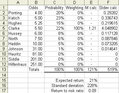
The problem with this formula is it involves a large number of variables. The best way to calculate the standard deviation, and in turn the optimal strategy, is to use spreadsheet software like Microsoft Excel. Below is a screenshot of the workings for the calculation of the standard deviation and return to risk ratio for a wager on Clarke.

To calculate expected return, column E calculates (probability * odds * weighting) for each outcome. Cell E13 sums these figures and cell E15 calculates the expected return, m, for a particular series of bets, by subtracting 1 from E13. Refer to the relevant formula above for clarification.
To calculate standard deviation, column F calculates probability * (odds * weighting – 1 – m)2 for each outcome. m equals the value in E15. Cell F13 sums these figures and cell E16 takes the square root to provide the standard deviation.
In the example above a bet on Clarke would have an expected return of 21% with a standard deviation of 228%. As mentioned before, this provides a reward to risk ratio of 21% / 228% = 0.09.
To calculate the combination of bets that provides the best reward to risk ratio, we need to use the Excel Solver feature. To make this feature available, select Tools -> Add-Ins in the menu bar. Select the Solver Add-In and click on OK. To use the solver, select Tools -> Solver.

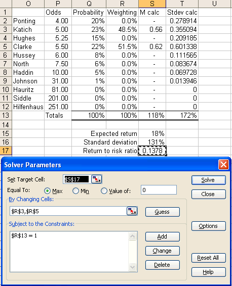
The Solver attempts to set a target cell equal to a certain value by manipulating other selected cells. For our purposes, Solver is used to find the maximum possible value for the return to risk ratio by manipulating the betting weights. The example in the screenshot below only manipulates the weights for Clarke and Katich because they are the only players that provide a positive expected return. Note that a constraint is set so that the sum of the weights equals 1.

By placing 48.5% of our wager on Katich and 51.5% on Clarke we have an expected return of 18% and a standard deviation of 131%. This provides a return to risk ratio of 0.14, which is a substantial improvement on 0.09 if we only backed Clarke. We have reduced our risk drastically and have only dropped the expected return from 21% down to 18%. This is a marked improvement on the maximising expected return strategy.
Based on the above example, if we wish to bet $100 on this market, our optimal strategy is to wager $48.50 on Katich and $51.50 on Clarke.
It is important to stress that this strategy is heavily dependent on the expected probabilities for each outcome. If you get these right then this strategy will pay handsome dividends. However, as the saying goes "garbage in, garbage out." If your expected probabilities are inaccurate then the execution of this, or any strategy, will lead to poor results.
|
<< Previous topic: Betting Suggestions |
Next topic: Staking Plans >> |
